From a Real-Valued Signal to the FFT and Its Spectrum

Introduction

Ever wondered how we turn a real-world signal, like audio, into its frequency components? In this post, we’ll dive into the Fast Fourier Transform (FFT), a powerful tool that converts a real-valued signal \(x[n]\) into its complex-valued frequency domain \(X[f]\). We’ll explore the math behind it, compute the FFT using Python libraries like NumPy and PyTorch, and visualize the spectrum to reveal the signal’s frequency content.

But before we dive in, let’s grab the essential tools.

import torch
import scipy
import numpy as np
import soundfile as sf
import matplotlib.pyplot as plt

From a Real-Valued Signal to the FFT and Its Spectrum

Let’s start with the definition. For a real-valued discrete-time signal \(x[n]\) of length \(N\), its Discrete Fourier Transform (DFT), often computed using the Fast Fourier Transform (FFT), is given by:

where

• \(x[n]\) is the input signal in the time domain (real-valued),
• \(X[f]\) is the complex-valued output in the frequency domain,
• \(j\) is the imaginary unit, where\(j^2 = -1\),
• \(N\) is both the number of time-domain samples and the number of frequency bins.

Computing FFT in Python

Let’s begin by loading our first audio signal. Start by downloading a file from this link, corresponding to a male speech signal from Librispeech corpus.

import soundfile as sf
signal, sr = sf.read('1221-135767-0010.wav')
print(signal.shape)
print(sr)

This signal has 131,200 samples and a sample rate of 16,000 Hz.

Now, we compute the fast Fourier transform (FFT) using either numpy, scipy or torch:

# Compute FFT using numpy
fft = np.fft.fft(signal)

# Compute FFT using scipy
fft = scipy.fft.fft(signal)

# Compute FFT using torch
signal_pt = torch.from_numpy(signal).float() # convert numpy to torch 
fft = torch.fft.fft(signal_pt)

print(fft.size)
>> 131200

Each method gives us an output of the same length (131200), corresponding to one frequency bin per time-domain sample. However, Minor numerical differences may arise : NumPy and SciPy’s output (e.g., -1756.95983887) shows higher decimal precision compared to PyTorch’s -1756.9597, reflecting slight differences in floating-point arithmetic or rounding conventions, likely due to PyTorch’s optimizations for GPU acceleration or performance efficiency.

Visualizing the FFT: Why Does It Look Mirrored?

plt.plot(fft)
plt.xlabel('Frequency (Hz)')
plt.ylabel('Amplitude')
plt.title('PyTorch FFT')
plt.show()

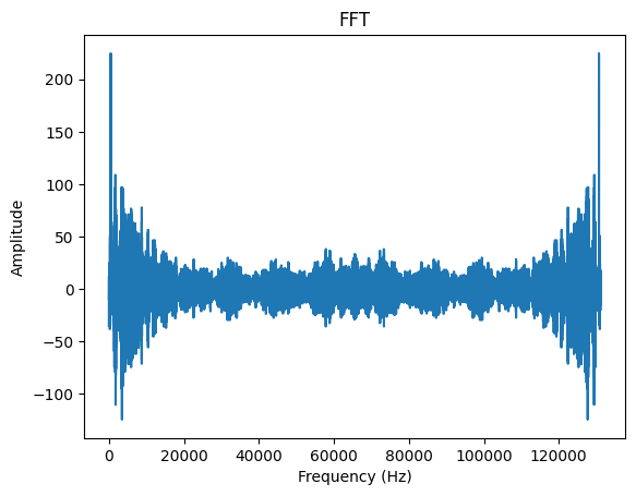
Why does the FFT output look mirrored — and can we simplify it by keeping only the useful part?

First of all, if you try to plot the full complex-valued FFT directly, you’ll encounter a ComplexWarning indicating that only the real part is being displayed while the imaginary part is discarded.

Furthermore, while this plot gives a complete view (of the real part) of the FFT output, it includes both positive and negative frequencies — leading to symmetric redundancy that’s often unnecessary for real-valued signals.

To this end, we retain only the first half of the frequency bins (from \(0\) to \(\frac{N}{2}\)) which correspond to the positive frequencies, and discard the second half (from \(\frac{N}{2}+1\) to \(N-1\)) which represent the negative ones.

Positive? Negative? I don’t quite see how the values on the left (or the first half) are “positive” and those on the right (the second half) are “negative”!

Well, I do agree that it’s not straightforward. Let’s break it down.

In fact, each frequency bin \(f\) in the FFT corresponds to a complex sinusoid with angular frequency \(\omega_f = \frac{2\pi f}{N}\).

If you remember our very first example, you might’ve noticed something interesting — a kind of symmetry in the FFT output.

In fact, it’s a general property known as Hermitian symmetry: for any real-valued time-domain signal, its FFT satisfies

Visualizing the Positive-Frequency FFT

To begin with, let’s plot the FFT while keeping only the positive frequencies (i.e., the left half) and discarding the negative ones on the right:

plt.plot(fft[:int(len(fft)/2)])
plt.xlabel('Frequency (Hz)')
plt.ylabel('Amplitude')
plt.title('Positive-Frequency FFT')
plt.show()

To sum up: when you plot the FFT directly (e.g., using plt.plot(fft)), Python raises a ComplexWarning because it only displays the real part — silently discarding the imaginary part. As a result, you lose half the information, and the plot may not accurately reflect the true frequency content (we’ll address this properly in the next section). Moreover, since the FFT of a real-valued signal includes both positive and negative frequencies — which are symmetric — we usually keep and display only the first half.

Computing and Vizualizing the Spectrum

Because complex numbers are hard to interpret visually, a common solution is to compute the magnitude, which combines information from both the real and imaginary parts. The magnitude of the FFT — known as the spectrum — is defined as:

This gives a complete measure of the amplitude at each frequency component. That’s why plotting \(\lvert X[f] \lvert\) is both more informative and widely used in practice.

Let’s plot everything. Let’s compute first the spectrum from the fft.

fft = scipy.fft.fft(signal)
spectrum = np.abs(fft)

Now let’s plot the spectrum directly and vizualize it.

plt.plot(spectrum)
plt.xlabel('Frequency (Hz)')
plt.ylabel('Amplitude')
plt.title('PyTorch FFT')
plt.show()

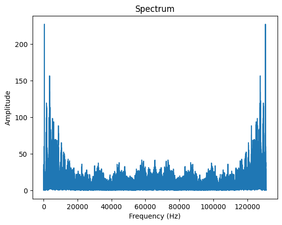
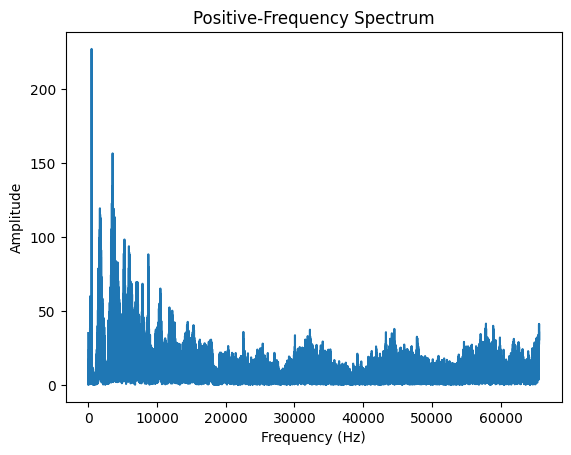
As explained previously, you notice a mirror effect corresponding to keeping both positive and negative values. Thus, we discard the negative values and keep only the positive values and we get it as follows:

plt.plot(spectrum[:int(len(fft)/2)])
plt.xlabel('Frequency (Hz)')
plt.ylabel('Amplitude')
plt.title('Positive-Frequency Spectrum')
plt.show()

A Practical Consideration for Visualization

Computing the FFT on a signal using the whole number of samples can be interesting and informative for some types of processing (e.g., pitch estimation or signal classification), but not ideal for visualization, as it produces a very high-resolution spectrum — one frequency bin per sample — and it averages out all temporal variations.

In such a full-FFT case, the number of frequency bins is equal to the number of samples (for real input: N/2 + 1). To visualize or reduce dimensionality, one might consider decimating the spectrum (e.g., keeping one frequency every k bins) or zooming into a limited frequency range, but these approaches can be lossy or arbitrary.

Importantly, if you compute the FFT on only the first n_fft samples of the full signal, you are discarding the rest of the signal, which is usually not appropriate, especially for non-stationary signals like speech. A better practice is to segment the signal into overlapping windows of length n_fft, compute the FFT on each (optionally windowed), and then average the magnitude or power spectra. This approach gives a more representative global spectrum and preserves temporal structure during analysis.

In fact, this is exactly what the short-time Fourier transform (STFT) does: it computes the FFT over short-time segments of the signal. If you don’t care about temporal variation and only want a global spectral profile, you can then average the STFT across time (i.e., average over frames), giving a smoothed and representative spectrum of the whole signal.

Conclusion

And that’s the magic of the FFT! We’ve journeyed from a real-valued signal to its frequency domain, using the FFT to uncover hidden frequency components. By computing the spectrum \(\lvert X[f] \rvert\), we get a clear, visual snapshot of a signal’s amplitude across frequencies. With Python tools like NumPy and PyTorch, and by focusing on positive frequencies, we’ve made sense of complex outputs in a practical way. This process is key in signal processing, helping us analyze everything from audio to vibrations with ease and precision. Keep exploring, and happy signal crunching!